Demo Page

The magnitude of the external field is displayed above the vectors of the sub-layer magnetizations (because of the normalisation of the modell, the external magnetic field, at which all the magnetic momenta are paralell to this external field is 4*J/M, where M is the layer magnetization and J is the bilinear coupling constant.

At the end of the presentation hints will be given on how to view the graphs at different view angles and displaying speed to get full understanding of the presentation.

If you would like to view the mentioned demos from different views and different speeds you must have `gnu-plot' installed on your system (with the so called `arrows' functionality -- for example Linux version 3.5 (pre 3.6) patch-level beta 347 -- and `less' for reading the text files. Should you not see moving arrows on the 3D plots your gnu-plot version is old and needs an update. If desperate, please download a suitable version of gnu-plot from the anonymous ftp site of nucssp.rmki.kfki.hu (.deb stands for Debian package, .rpm for Red Hat package). Installation under Debian: dpkg -i NAME.deb (as root), under Red Hat: rpm -i NAME.rpm (also as root).

In the presentation above, the system consisted of 10 magnetic layers, and had a first-neighbor anti-ferromagnetic coupling. It means, that the energy function of the system is:

theta=(theta[0],theta[1],...,theta[9]),

                    /  9   /  9                                   \\
                    |----- |-----                                 ||
                    | \    | \                                    ||
H(theta):=    - 1/2 |  )   |  )   J[i, j] cos(theta[i] - theta[j])||-
                    | /    | /                                    ||
                    |----- |-----                                 ||
                    \j = 0 \i = 0                                 //


         /  9                     \
         |-----                   |
         | \                      |
     - h |  )   M[i] cos(theta[i])|
         | /                      |
         |-----                   |
         \i = 0                   /

Where M[i] the i-th magnetic moment, J[i,j] the coupling constant and h the external magnetic field. In this simulation all the J[i,i+1]=J[i,i-1]=-1,J[i,j]=0 (if j<>i+1 and j<>i-1), M[i]=1, thus the external magnetic field when cos(theta[i])=1 (all the momenta are paralell to the field) will be at maximum 4 units (and not less than 2 units).

---

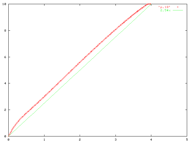
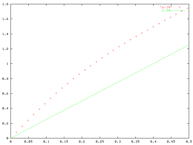
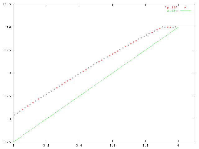
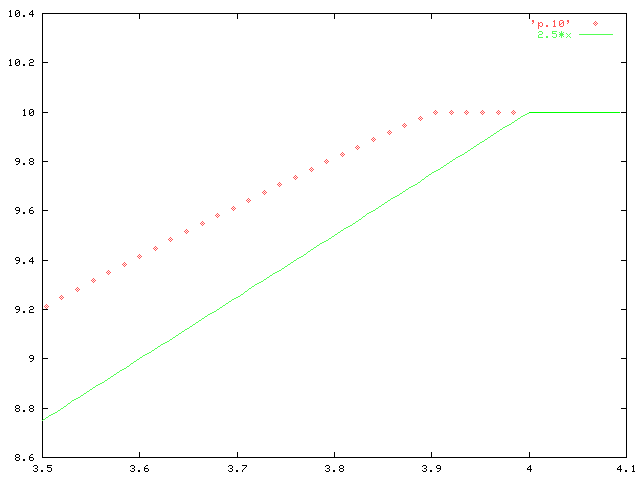
In the next set of plots the net magnetization of the system (red diamonds) is plotted as a function of the external magnetic field (in arbitrary units).

---

---

The straight green line is the predicted value of magnetization from the two sublayer model (with infinite number of layers, i.e. with periodic boundary conditions).

The different ranges of magnetic field can be seen below. On the zoomed graphs you will see, that the 'real' magnetization (of the finite system) is always higher than that of the infinite system (because the top and the bottom moments incline to a higher extent towards the magnetic field)

---

---

Now let's see a bigger system of 64 magnetic layers! Please watch closely the top three and the bottom three layers which behave 'anomalously'. Please note the 'wavelike' 'twisted' arrangement in small external fields.

---

There is a demo (mentioned in the begining of the document) available if you have the appropriate version of gnuplot. You can download demo.zip from the anonymous ftp of nucssp. After unzipping the file, start demo (but first give righ to run: chown u+x demo).

Also now you can view the plots without running the demo. To do so, start gnu-plot, then enter two variables as follow:

  gnuplot> layer=10 (or 64 depending on the file, you want
                     to view)
  gnuplot> ido=0 (or -1)  this variable sets the time between
                          the frames: -1 means you must hit 
                          ENTER after each frame. NB! you first 
			  must activate the x-term window, and
			  then hit the ENTER (not when the plot
			  window is active)!

  gnuplot> load 'init'
And now for the 3D plot:
  gnuplot> load 'pv.10' (or 'pv.64' respectively)
To change the view, use `set view xangle, zangle'
  gnuplot> set view 0,0
Then use replot to view the result:
  gnuplot> replot

  gnuplot> plot 'p.10' (or p.64')
for the magnetization and
  gnuplot> plot 'p.10' using 1:3
for the energy versus external magnetic field plot.

Also you can plot other functions with the data, for example
  gnuplot> plot 'p.10' using 1:3, -x**2
And you can select the region you want to plot by
  gnuplot> plot [0:1] [-15:0] 'p.10' using 1:3, -x**2
For further details, please refer to gnu-plot's help
  gnuplot> help